To qualify the ADS1211 for the given application, or at least, to gain some confidence in it, a test – not the for overall non-linearity (i.e., non-linearity over the full range, aka integral nonlinearity INL), but for the more detailled view at the ADC’s precision.
Local deviation of an ADC from linearity are called differential linearity, and this can be some slight deviation, or can go so far that there are even “missing codes”. A missing code is caused by a local non-linearity that is larger than 1 LSB, to the ADC will jump 2 steps, even if the voltage is only increased by 1 LSB equivalent.
First, the test setup: still the ADS1211, running at 4 MHz, 16 turbo mode, 60 Hz data rate. Connected by fully-differential coax to a (floating) source, an HPAK 8904A signal generator. This is programmed for a 5 DV output, with 20 mVpp (intentional) sine ripple, 13 Hz. The selection of the frequency is rather critical, don’t let it be anywhere close to a subharmonic or harmonic of the data rate!
The HPAK 8904A is actually really great for this purpose, you can add and mix any signals, up to 4 channels, and modulations, as desired, into one channel!
Alternatively, you could feed DC-biased noise, but these noise signals can be troublesome, and you never now what to expected in terms of amplitude, flatness, etc, unless you have really specialized gear.
Having everything set up, several hours of data were collected. Virtually no drift, so the DC component-the average ADC code (nearest integer) was subtracted from the data, and the results analyzed.
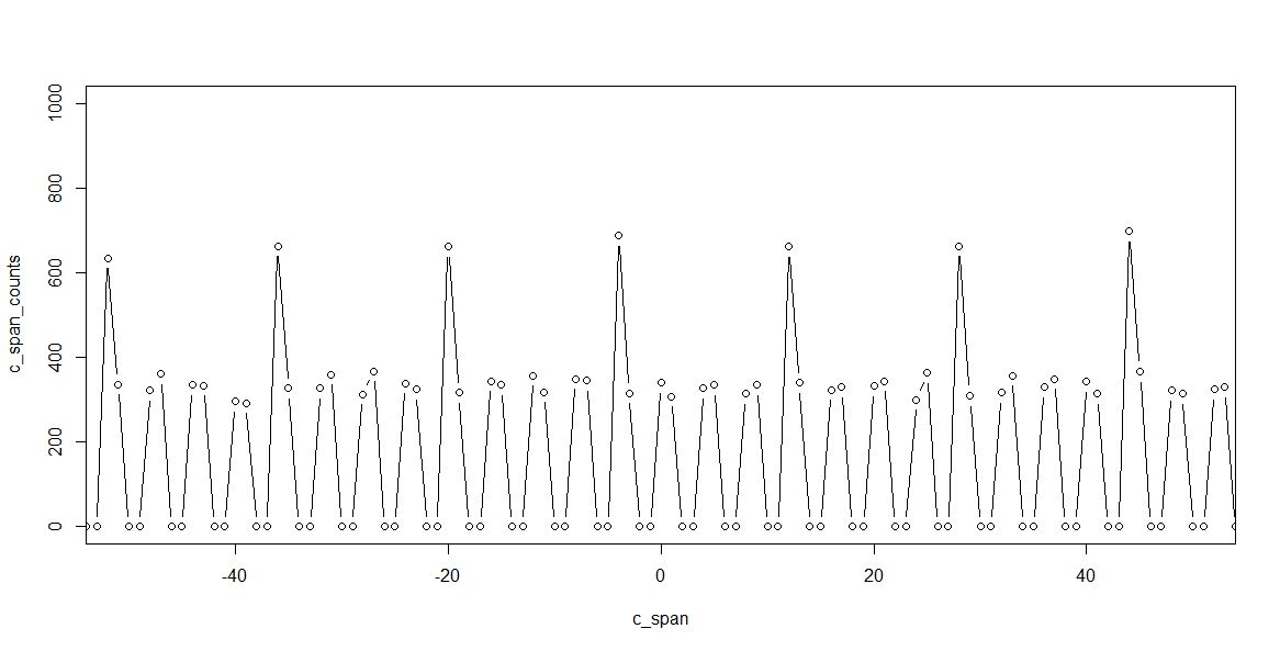
Full data, +-2000 counts is more or less +-10 mV (20 mVpp), as expected. 1 LSB is about 4 µV. There is dot for every count, even if no sample was recorded, at the given count (then, the dot is at 0 samples…).
The probability density function (PDF) corresponds to that of a sine function. That’s a good start.
Some key observations – there seem to be 3 “populations” of sample counts – codes that are “0”, i.e., missing codes; codes that have counts that are somewhat in-between (the majority), and double-counting codes. This needs some more investigation.
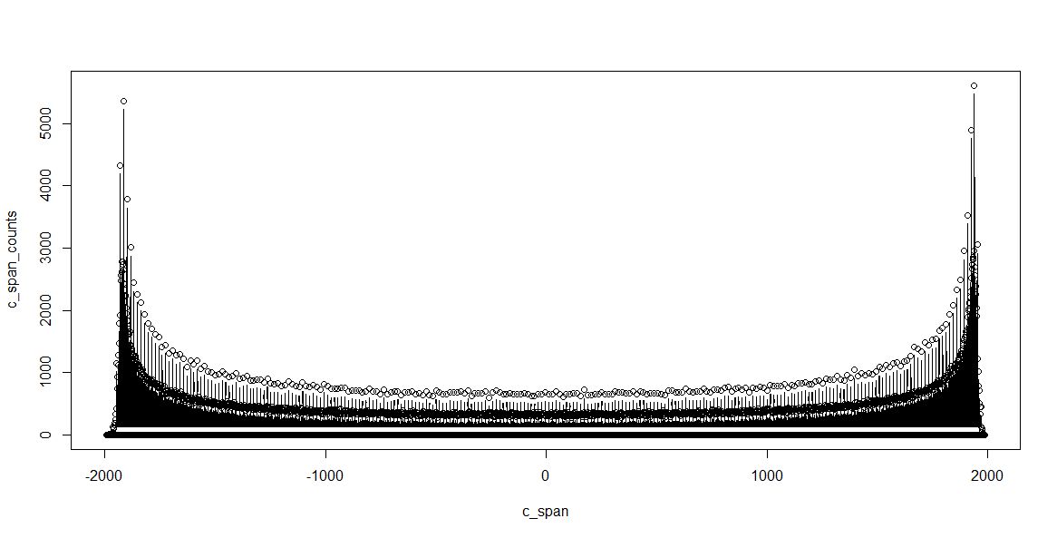
Taking all these data, and the know PDF of sine (of the form, 1/(x*(1-x), “bathtub curve”), the PDF was fit to the data, using least squares.
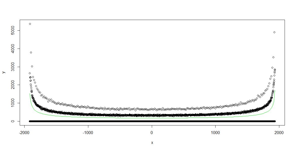
Green line shows the fit-this makes sense, and the residuals were calculated.
We are only interested in the center part, where the errors due to drift are minimal. A close up:
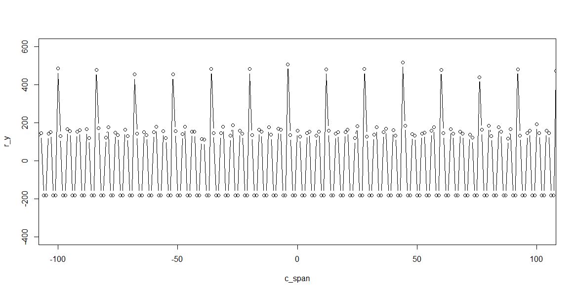
We can cleary see a pattern: DxMMxxMMxxMMxxMMDxMMxxMMxxMMxxMMD…
D – double code, M – missing, x – intermediate.
What seems dramatic, it’s acutally not. There aren’t any deviations more than +-1 LSB, and there will be noise and averaging anyway, to get beyond even 22 bit resolution.